
Unlike previous methods of Interpolating,
Spline interpolation does not produce the same unique interpolating polynomial, as with the Lagrange method, Vandermonde matrix method, or Newton’s divided difference method. Spline interpolation addresses some of the error concerns of polynomial interpolation: low-degree polynomial interpolation can give poor approximations, while high-degree interpolating polynomials may introduce large over-correcting oscillations. Spline interpolation uses multiple lower-degree polynomials, such that high-order error is reduced. Because each spline is also using fewer terms, problems arising from using a large number of data points, such as vanishing determinants in Vandermonde matrices, can be avoided. Cubic splines create a series of piecewise cubic polynomials.
For n+1 data points:

The interpolating splines are as follows:
![S(x) = \left\{\begin{matrix} S_0(x) & x \in [x_0, x_1] \\ S_1(x) & x \in [x_1, x_2] \\ \vdots & \vdots \\ S_{n-1}(x) & x \in [x_{n-1}, x_n] \end{matrix}\right.](https://s0.wp.com/latex.php?latex=S%28x%29+%3D+%5Cleft%5C%7B%5Cbegin%7Bmatrix%7D+S_0%28x%29+%26+x+%5Cin+%5Bx_0%2C+x_1%5D+%5C%5C+S_1%28x%29+%26+x+%5Cin+%5Bx_1%2C+x_2%5D+%5C%5C+%5Cvdots+%26+%5Cvdots+%5C%5C+S_%7Bn-1%7D%28x%29+%26+x+%5Cin+%5Bx_%7Bn-1%7D%2C+x_n%5D+%5Cend%7Bmatrix%7D%5Cright.+&bg=ffffff&fg=333333&s=1&c=20201002)
Where

Which is simplified by using the substitution 

To guarantee the smooth continuity of the interpolating Spline 
1) 
2) 
3) 
4) 
As stated on the Wikipedia page, the first requirement imposes n+1 restrictions, while requirements 2,3,4 impose n-1 restrictions each, for a total n+1 + 3(n-1) = 4n-2. Because we are finding 4 coefficients for each of n polynomials, we need 4n restrictions. Clamped splines use fixed bounding conditions for 


We will use these 4 rules and 2 bound conditions to construct a tri-diagonal matrix which can be efficiently solved, giving the coefficients of each spline.
Ensuring Rule 2:
First, the simple form of 

Rules 1 and 2 together give us:
Combining these two equations gives us:

Since 

Where
Ensuring Rule 3:
Next, we ensure first derivatives match:
Taking the derivative of the simple form of a spline, we have:
We combine 


Ensuring Rule 4:
We repeat step 2, but for the second derivative, using:


We are ensuring rule 4:
Combining these, we have:

Giving:

Solving for  :
:
With our bound conditions 


First we solve Eq.1 for 


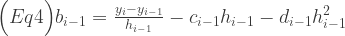

Next, we rearrange Eq.3:

Multiply both sides by 
Next, solve Eq.2 for the d term as follows:

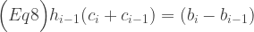
Substitute this into the right-hand side of Eq.6 to get:

Move the c term from the right side to the left:

Combine like terms on the left side to get:
By substituting Eq.4 (for 

Moving both c terms to the left gives:

The 

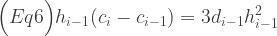
Now we solve Eq.6 for 
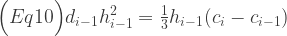
And for 

We can substitute Eq.10 and Eq.11 into Eq.9 and factor the 


Multiplying by 3 to remove fractions and moving the 

Combining like terms on the left:

And finally expressing the left as a combination of c:

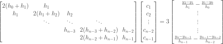
We can now express this as a tri-diagonal matrix times c and using an efficient recursive method to solve the tri-diagonal, get the values of c:
Solving the remaining coefficients:
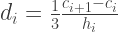
With c known, we can easily calculate the remaining coefficients:
We solve Eq.3 for 

We know that 

Finally, we can calculate 
Code + Example:
This python code has a function Spline(data) that takes a set of ordered x,y pairs and returns a list of tuples, where each tuple represents the values 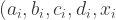

In both images, the red dashed line represents the Cubic Spline interpolation, while the solid blue line is the Lagrange interpolating polynomial. In the first image, the black line is the actual function.


